Object Detection Challenges:
- Intra class variance
- Pose variation
- Occlusion / Large search space over multiple: (a) Location, (b) Scale, (c)Aspect ratio;
- Crowded scenes
Traditional Object Detection Pipeline:
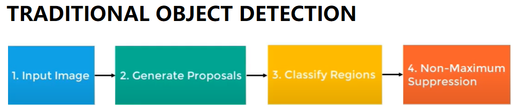
- Input image;
- Generate proposals:
- Background substraction;
- Sliding windows with scales;
- Selective search:
- adds all boundary boxes to the list of region proposed;
- groups adjacent segments based on similarity;
- Classify Regions:
- HOG/SURF + SVM/RF/ADABOOST
- Non-maximum suppression.
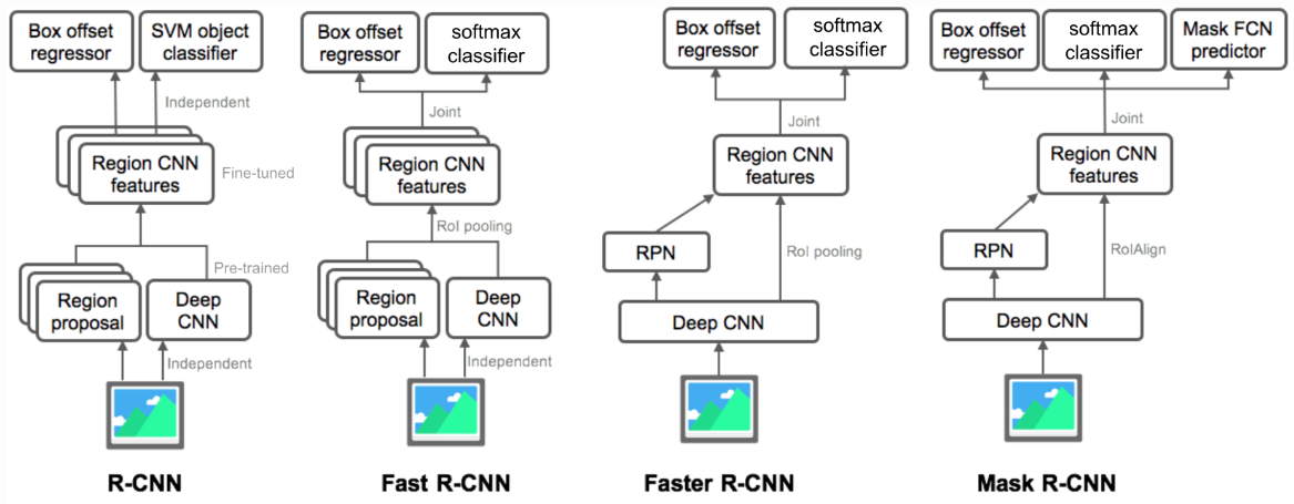
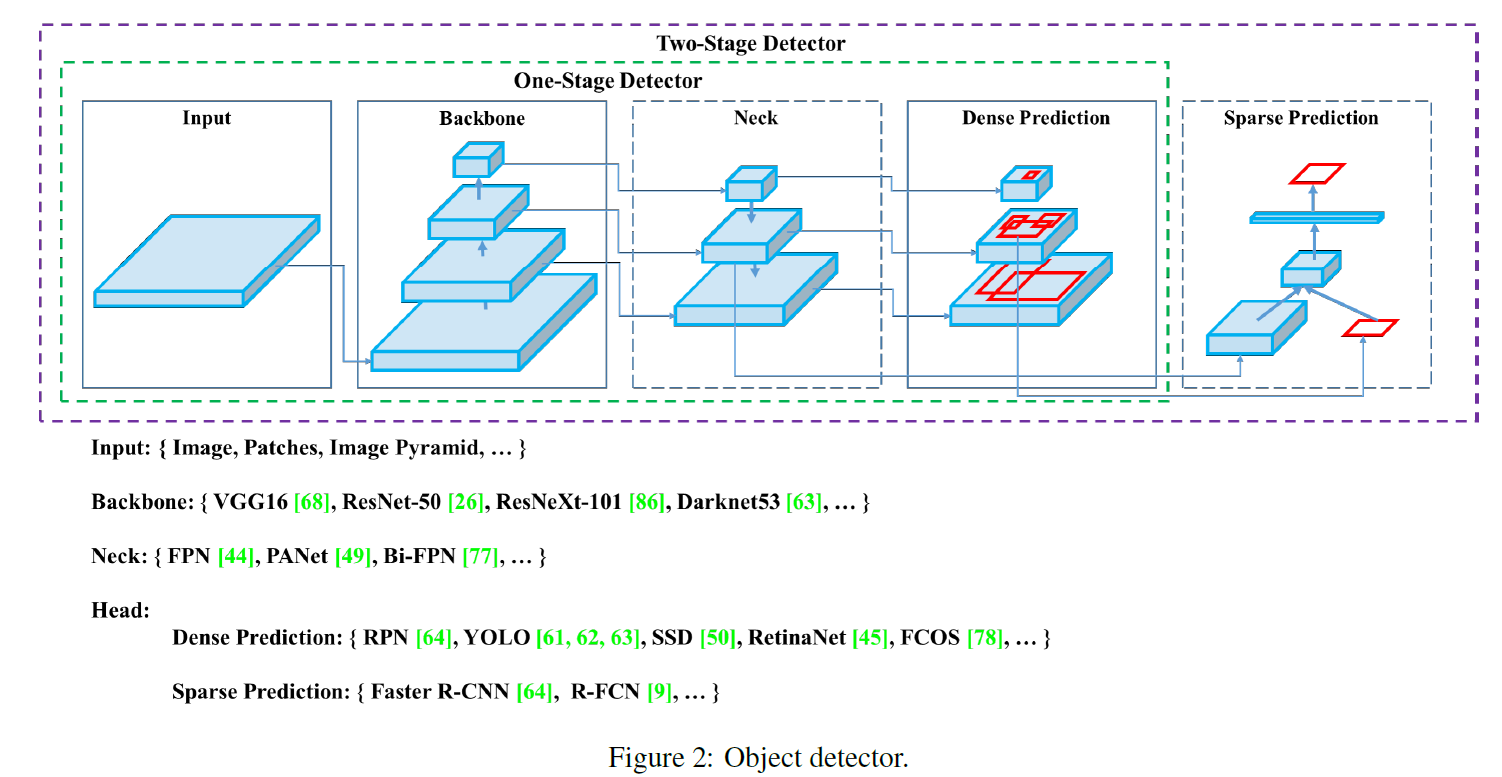
Two Stage Object Detection (RCNN Family):
- Proposal generator: Extract bounding box from images; (not need to be NN, but should be smart);
- Refine module: Classify and redefines bounding box; (trainable module that uses the visual feature to refine the module).
| Model | Paper | code |
|---|---|---|
| R-CNN | [paper] | [code] |
| Fast R-CNN | [paper] | [code] |
| Faster R-CNN | [paper] | [code] |
| Mask R-CNN | [paper] | [code] |
R-CNN’s
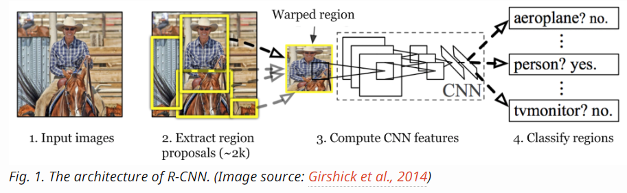
Model Workflow:
- Pre-train a CNN network on image classification tasks; for example, VGG or ResNet trained on ImageNet dataset. The classification task involves N classes.
- Propose category-independent regions of interest by selective search (~2k candidates per image). Those regions may contain target objects and they are of different sizes.
- Region candidates are warped to have a fixed size as required by CNN.
- Continue fine-tuning the CNN on warped proposal regions for K + 1 classes; The additional one class refers to the background (no object of interest). In the fine-tuning stage, we should use a much smaller learning rate and the mini-batch oversamples the positive cases because most proposed regions are just background.
- Given every image region, one forward propagation through the CNN generates a feature vector. This feature vector is then consumed by a binary SVM trained for each class independently. The positive samples are proposed regions with IoU (intersection over union) overlap threshold >= 0.3, and negative samples are irrelevant others.
- To reduce the localization errors, a regression model is trained to correct the predicted detection window on bounding box correction offset using CNN features.
Common tricks:
- Non-Maximum Suppersion
- Hard negative Mining
Its problem:
- interference of each ROI is done independently;
- R-CNN trains each independent part (CNN feature extractor, SVM classifier, Bounding Box Regressor) separately;
- Limitation of selective search algorithm as proposal generator (not trainable).
Fast R-CNN:
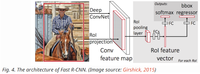
Model Workflow:
- Pre-train a convolutional neural network on image classification tasks.
- Propose regions by selective search (~2k candidates per image).
- Alter the pre-trained CNN:
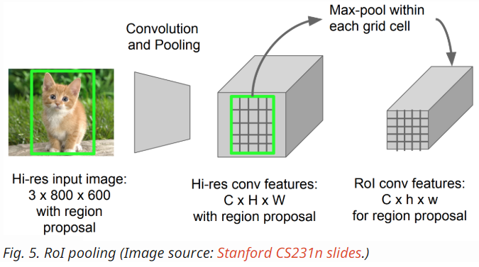
- Replace the last max pooling layer of the pre-trained CNN with a RoI pooling layer. The RoI pooling layer outputs fixed-length feature vectors of region proposals. Sharing the CNN computation makes a lot of sense, as many region proposals of the same images are highly overlapped.
- Replace the last fully connected layer and the last softmax layer (K classes) with a fully connected layer and softmax over K + 1 classes.
- Finally the model branches into two output layers:
- A softmax estimator of K + 1 classes (same as in R-CNN, +1 is the “background” class), outputting a discrete probability distribution per RoI.
- A bounding-box regression model which predicts offsets relative to the original RoI for each of K classes.
- ROI Pooling:
- ROI pooling converts a projected region to a fixed sized region;
- It applies Max Pooling for each region.
- Loss function: classification loss (cross entropy) + Localization loss (smooth L1)
More efficient, and can be trained in a single step in an end-to-end manner. But still non trainable selective search as proposal generator.
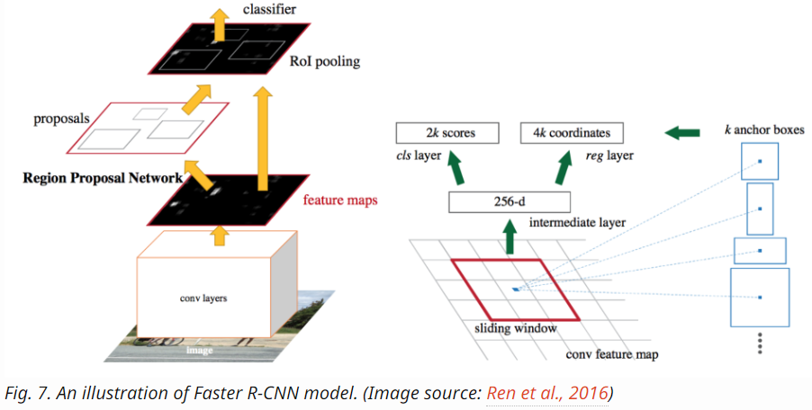
Faster R-CNN:
 Workflow:
- Pre-train a CNN network on image classification tasks.
- Fine-tune the RPN (region proposal network) end-to-end for the region proposal task, which is initialized by the pre-train image classifier. Positive samples have IoU (intersection-over-union) > 0.7, while negative samples have IoU < 0.3.
- Slide a small n x n spatial window over the conv feature map of the entire image.
- At the center of each sliding window, we predict multiple regions of various scales and ratios simultaneously. An anchor is a combination of (sliding window center, scale, ratio). For example, 3 scales + 3 ratios => k=9 anchors at each sliding position.
- Train a Fast R-CNN object detection model using the proposals generated by the current RPN
- Then use the Fast R-CNN network to initialize RPN training. While keeping the shared convolutional layers, only fine-tune the RPN-specific layers. At this stage, RPN and the detection network have shared convolutional layers!
- Finally fine-tune the unique layers of Fast R-CNN
- Step 4-5 can be repeated to train RPN and Fast R-CNN alternatively if needed.
- Region Proposal Network as a proposal generator:
- Each pixel of the feature map of the deep layer of CNN is a projection of some region of the input image;
- Area of RPN depends upon the receptive field of CNN;
- RPN is a trainable sliding window approach.
- Shared computation of CNN features;
- ROI pooling to convert features from proposed region to fixed size;
- Joint training of Boundning Box offset and classifier with CNN fine-tune.
- Loss function: classification loss (cross entropy) + Localization loss (smooth L1)
Recall:
One Stage Object Detection:
| Model | Paper |
|---|---|
| SSD | [paper] |
| YOLO v1 | [paper] |
| YOLO v2/9000 | [paper] |
| YOLO v3 | [paper] |
| RetinaNet | [paper] |
| YOLO v4 | [paper] |
SSD
SSD = (feature extractor) VGG-16 on ImageNet + (downsampling/pyramid representation) extra conv feature layers of decreasing sizes.
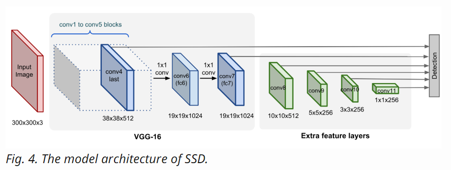 Pyramid image Intuitively: large fine-grained feature maps at earlier levels are good at capturing small objects and small coarse-grained feature maps can detect large objects well.
Workflow:
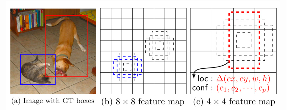
SSD does not split the image into grids of arbitrary size but predicts offset of predefined anchor boxes for every location of the feature map. Each box has a fixed size and position relative to its corresponding cell. All the anchor boxes tile the whole feature map in a convolutional manner.
In SSD, the detection happens in every pyramidal layer. Feature maps at different levels have different receptive field sizes. The anchor boxes on different levels are rescaled so that one feature map is only responsible for objects at one particular scale. For example, in Fig below the dog can only be detected in the 4x4 feature map (higher level) while the cat is just captured by the 8x8 feature map (lower level).
 At every location, the model outputs 4 offsets and c class probabilities by applying a 3×3×p conv filter (p is the number of channels in the feature map) for every one of k anchor boxes.
Loss Function: Loss = Localization loss (smooth L1) + Classification loss (softmax cross entropy with logits). SSD uses hard negative mining to select easily misclassified negative examples to construct this neg set: Once all the anchor boxes are sorted by objectiveness confidence score, the model picks the top candidates for training so that neg:pos is at most 3:1.
YOLO v1
Does not have Proposal Generator and Refine Stages, but directly predicts Bounding Box through Single Stage Network using features from the entire image and predicts Bounding Box of all classes simultaneously. (Model is similiar to classification nets).
Workflow:
- Pre-train a CNN network on image classification task.
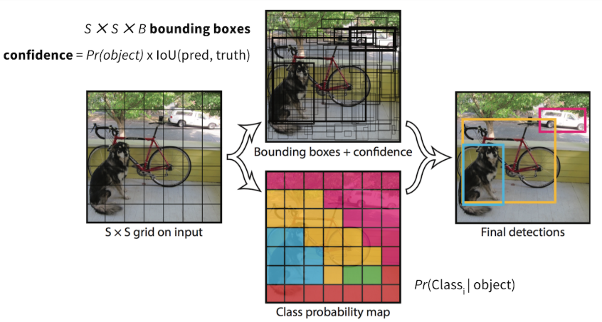
- Split an image into S×S cells. If an object’s center falls into a cell, that cell is “responsible” for detecting the existence of that object.
- coordinates: A tuple of 4 values (x, y, w, h);
- confidence score:
Pr(containing an object) x IoU(pred, truth);
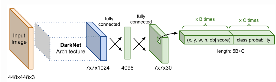
- Final layer of the pre-trained CNN is modified to output a prediction tensor of size S×S×(5B+K).
Network:
The final prediction of shape S×S×(5B+K) is produced by two fully connected layers over the whole conv feature map.
YOLO training:
- Cells contain the center if the ground truth bounding box is responsible for detecting it.
- Adjust the cell’s label to “car”;
- Find the predicted bounding box:
- Increase confidence of bouning box with largest overlap with GT;
- Decrease confidence of bouning box with smaller overlap.
- Cells do not contain an object:
- Reduce confidence of bounding boxes;
- Do not change class probabilities or bounding box coordinates.
Loss function:
- Localization error; (Original centers & Width & Height) (If an object is present, minimize loss function only when there is an object presenting in the bounding box).
- The loss function only penalizes classification error if an object is present in that grid cell, 1_obj_i = 1;
- The loss function only penalizes bounding box coordinate error if that predictor is “responsible” for the ground truth box, 1_obj_ij=1.
- Confidence of the bounding box;
- Confidence of the bounding box at empty cells;
- Conditional probability of final class.
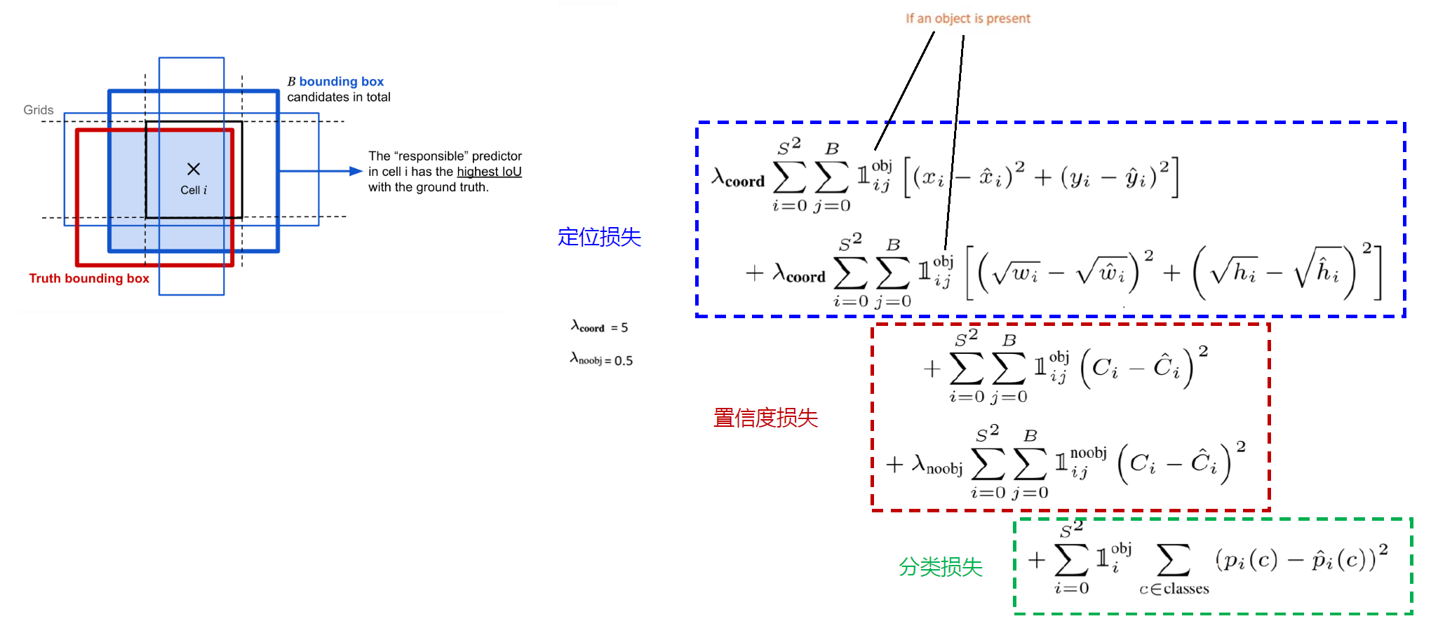 At one location, in cell i, the model proposes B bounding box candidates and the one that has highest overlap with the ground truth is the “responsible” predictor.
YOLO v2/ YOLO9000
Improvements
- BatchNorm: helped a bit over convergence;
- Image resolution: fine-tuning the base model with high resolution images;
- Convolutional anchor box detection: Rather than predicts the bounding box position with fully-connected layers over the whole feature map, YOLOv2 uses convolutional layers to predict locations of anchor boxes, like in faster R-CNN.
- K-mean clustering of box dimentions: Different from faster R-CNN that uses hand-picked sizes of anchor boxes, YOLOv2 runs k-mean clustering on the training data to find good priors on anchor box dimensions;
- Direct location prediction;
- Add fine-grained features: similar to identity mappings in ResNet to extract higher-dimensional features from previous layers;
- Multi-scale training: a new size of input dimension is randomly sampled every 10 batches;
- Light-weighted base model: DarkNet-19.
YOLO9000: Rich Dataset Training
Because drawing bounding boxes on images for object detection is much more expensive than tagging images for classification, the paper proposed a way to combine small object detection dataset with large ImageNet so that the model can be exposed to a much larger number of object categories. The name of YOLO9000 comes from the top 9000 classes in ImageNet. During joint training, if an input image comes from the classification dataset, it only backpropagates the classification loss.
In order to efficiently merge ImageNet labels (1000 classes, fine-grained) with COCO/PASCAL (< 100 classes, coarse-grained), YOLO9000 built a hierarchical tree structure with reference to WordNet so that general labels are closer to the root and the fine-grained class labels are leaves. In this way, “cat” is the parent node of “Persian cat”.
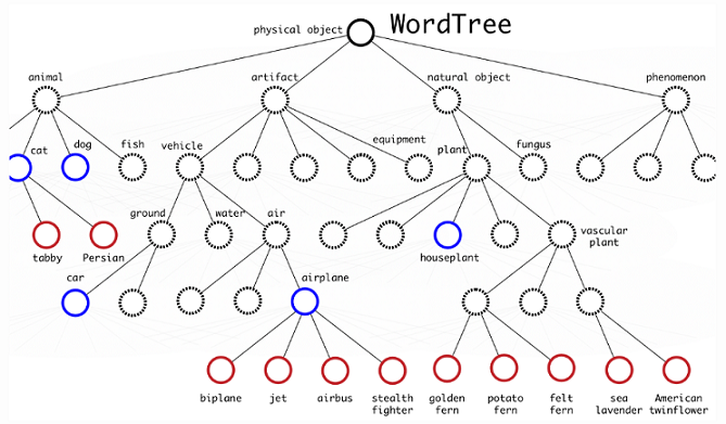 To predict the probability of a class node, we can follow the path from the node to the root:
1
2
3
4
5
Pr("persian cat" | contain a "physical object")
= Pr("persian cat" | "cat")
  Pr("cat" | "animal")
  Pr("animal" | "physical object")
  Pr(contain a "physical object")    # confidence score.
Note that Pr(contain a “physical object”) is the confidence score, predicted separately in the bounding box detection pipeline. The path of conditional probability prediction can stop at any step, depending on which labels are available.
YOLO pros and cons:
- much faster than Faster R-CNN, and v3 reached very good accuracy;
- Hard to detect groups of small objects (limited number of boxes);
- Hard to handle multi-scale objects (limited scale of output feature map).
YOLO v3
Improvements:
- Logistic regression for confidence scores: YOLOv3 predicts an confidence score for each bounding box using logistic regression, while YOLO and YOLOv2 uses sum of squared errors for classification terms. Linear regression of offset prediction leads to a decrease in mAP.
- No more softmax for class prediction: When predicting class confidence, YOLOv3 uses multiple independent logistic classifier for each class rather than one softmax layer. This is very helpful especially considering that one image might have multiple labels and not all the labels are guaranteed to be mutually exclusive.
- Darknet + ResNet as the base model: The new Darknet-53 still relies on successive 3x3 and 1x1 conv layers, just like the original dark net architecture, but has residual blocks added.
- Multi-scale prediction: Inspired by image pyramid, YOLOv3 adds several conv layers after the base feature extractor model and makes prediction at three different scales among these conv layers. In this way, it has to deal with many more bounding box candidates of various sizes overall.
- Skip-layer concatenation: YOLOv3 also adds cross-layer connections between two prediction layers (except for the output layer) and earlier finer-grained feature maps. The model first up-samples the coarse feature maps and then merges it with the previous features by concatenation. The combination with finer-grained information makes it better at detecting small objects.
Interestingly, focal loss does not help YOLOv3, potentially it might be due to the usage of λ_noobj and λ_coord — they increase the loss from bounding box location predictions and decrease the loss from confidence predictions for background boxes.
YOLO v3 on Darknet and OpenCV
- Initialize the parameters:
(a). Confidence threshold. Every predicted box is associated with a confidence score. In the first stage, all the boxes below the confidence threshold parameter are ignored for further processing.
(b). Non-maximum suppression threshold. The rest of the boxes undergo non-maximum suppression which removes redundant overlapping bounding boxes.
(c). Input Width & Height. 416 for default, but can also change both of them to 320 to get faster results or to 608 to get more accurate results. - Load model and classes:
(a). coco.names contains all the objects for which teh model was trained;
(b). yolov3.weights pre-trained weights;
(c). yolov3.cfg configuration file.
OpenCV DNN module set to use CPU by default, but we can setcv.dnn.DNN_TARGET_OPENCLfor Intel GPU. - Process each frame:
(a). Getting the names of output layers: The forward function in OpenCV’s Net class needs the ending layer till which it should run in the network. Since we want to run through the whole network, we need to identify the last layer of the network by usinggetUnconnectedOutLayers()that gives the names of the unconnected output layers, which are essentially the last layers of the network. Then we run the forward pass of the network to get output from the output layers, as in the previous code snippet(net.forward(getOutputsNames(net))).
(b). Draw the predicted boxes;
(c). Post-processing the network’s output:
The network outputs bounding boxes are each represented by a vector of number of classes + 5 elements. The first 4 elements represent the center_x, center_y, width and height. The fifth element represents the confidence that the bounding box encloses an object. - Main loop:
blobFromImage function scales the image pixel values to a target range of 0 to 1 using a scale factor of 1/255. It also resizes the image to the given size of (416, 416) without cropping. Keeping the swapRB parameter to its default value of 1.
See github ReadMe for more step-by-step training details: vince’s github
YOLO v4
YOLO v4 makes an object detector which can be trained on a single GPU with a smaller mini-batch size. This makes it possible to train a super fast and accurate object detector. To achieve this, v4 combined some features such as Weighted-Residual-Connections (WRC), Cross-Stage-Partial-connections (CSP), Cross mini-Batch Normalization (CmBN), Self-adversarial-training (SAT) and Mish-activation, Mosaic data augmentation, DropBlock regularization, and CIoU loss.
The methodology of objector detection:
There are no updates on the network artchitecture, but strategies to train the objector:
-
Bag of freebies: training strategies, no extra cost but accuracy improvement on test
a. data augmentation: Geometrical Transformaion, CutOut, Grid Mask
b. regularization: DropOut, DropBlock
c. class imbalance
d. hard sample 挖掘方法
e. 损失函数的设计 -
Bag of specials: increasing test cost a little, but significantly increasing accuracy
a. 增大模型感受野: SPP、ASPP、RFB
b. attention model: Squeeze-and-Excitation (SE)
c. spatial attention module (SAM)
d. 特征集成方法: SFAM , ASFF , BiFPN
e. 改进的激活函数: Swish、Mish
f. postprocess: soft NMS、DIoU NMS
The YOLOv4 could consists of:
Backbone: CSPDarkNet 53
Neck: SPP, PAN
Head: YOLO v3
RetinaNet
The RetinaNet is a one-stage dense object detector. Two crucial building blocks are featurized image pyramid (hierachical structure of converts to create feature maps) and the use of focal loss.
Focal loss: One of the bottlenecks of object detection is an extreme class imbalance between background that contains no object and foreground that holds objects of interests. Focal loss is designed to assign more weights on hard, easily misclassified examples (i.e. background with noisy texture or partial object) and to down-weight easy examples (i.e. obviously empty background).
Featurized Image Pyramid:
The featurized image pyramid (Lin et al., 2017) is the backbone network for RetinaNet. Following the same approach by image pyramid in SSD, featurized image pyramids provide a basic vision component for object detection at different scales.
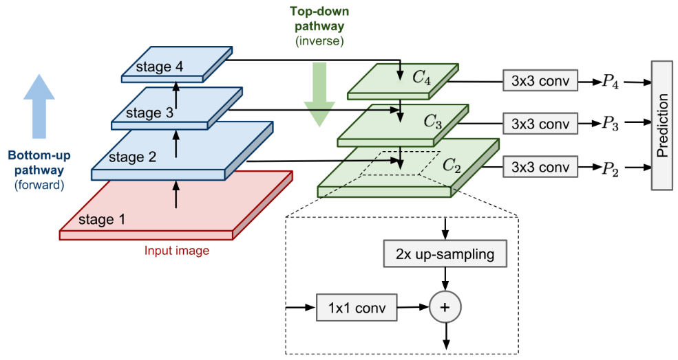
- Bottom-up pathway is the normal feedforward computation.
- Top-down pathway goes in the inverse direction, adding coarse but semantically stronger feature maps back into the previous pyramid levels of a larger size via lateral connections.
- First, the higher-level features are upsampled spatially coarser to be 2x larger. For image upscaling, the paper used nearest neighbor upsampling. While there are many image upscaling algorithms such as using deconv, adopting another image scaling method might or might not improve the performance of RetinaNet.
- The larger feature map undergoes a 1x1 conv layer to reduce the channel dimension.
- Finally, these two feature maps are merged by element-wise addition.
Model Architecture:
The featurized pyramid is constructed on top of the ResNet architecture. Recall that ResNet has 5 conv blocks (= network stages / pyramid levels).
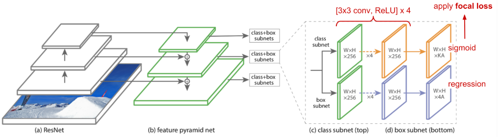 As usual, for each anchor box, the model outputs a class probability for each of K classes in the classification subnet and regresses the offset from this anchor box to the nearest ground truth object in the box regression subnet. The classification subnet adopts the focal loss introduced above.
Also many thansk for @weng2017detection3’s blog: “http://lilianweng.github.io/lil-log/2017/12/31/object-recognition-for-dummies-part-3.html”