Single Stage Object Detection

The pipeline to create a custom single stage detector:

1. Single-stage NN architecture 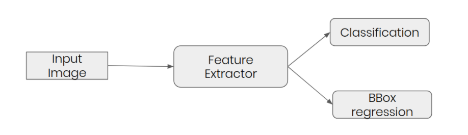As the network pipeline, the feature extractor is going to be the combination of ResNet-18 (pre-trained) and FPN (extract features from different layers). After that, two predictor: class predictor and bounding-box regressor.

2. generate anchor-boxes
Because of the feature extraction, the convolution feature of dimensions is: [num_channels, h, w]. The feature maps correspond to the position [:,i,j] ∀ i & j, use to have different bounding boxes (of different sizes and aspect ratios assuming this position is the center of the bounding box) associated with it. This predefined bounding box is called an anchor.

3. match prediction with ground truth
Predicting bounding boxes and class for each bounding box for every feature map. Encoding Boxes and Decoding Boxes.

4. loss function

5. training pipeline

Detector NN achitecture

I will use the Feature Pyramid Network for feature extraction. On top of this, I used class subnet and box subnet to get classification and bounding box.

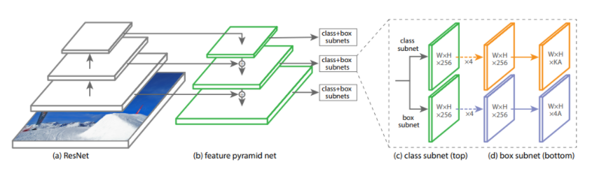FPN is built on top of ResNet (ResNet-18) in a fully convolutional fashion. It includes two pathways: bottom-up & top-down. These two pathways are connected in-between with lateral connections.

Bottom-up: forward path for feature-extracting.
Top-down: features closer to the input image have a rich segment (bounding box) information. So it is needed to merge all of the feature maps from different levels of the pyramid into one semantically-rich feature map.

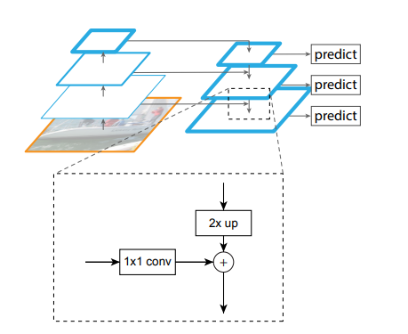
The higher-level features are upsampled to be 2x larger. For this purpose, nearest neighbor upsampling is used. The larger feature map undergoes a 1x1 convolutional layer to reduce the channel dimension. Finally, these two feature maps are added together in element-wise manner. The process continues until the finest merged feature map is created.

These merged features map goes into two different CNN of classes and bounding boxes predictions.

1.ResNet

import torch
import inspect
from torchvision import models
from IPython.display import Code
from fpn import FPN
from detector import Detector

resnet = models.resnet18(pretrained=True) 

The ResNet18 has the following blocks:

conv1
bn1
relu
maxpool
layer1
layer2
layer3
layer4
avgpool
fc

I used 1-8 blocks in FPG. But we take a look at the ouput dimension from these blocks:

# btch_size = 2, image dimesion = 3 x 256 x 256 

image_inputs = torch.rand((2, 3, 256, 256))

x = resnet.conv1(image_inputs)
x = resnet.bn1(x)
x = resnet.relu(x)
x = resnet.maxpool(x)
layer1_output = resnet.layer1(x)
layer2_output = resnet.layer2(layer1_output)
layer3_output = resnet.layer3(layer2_output)
layer4_output = resnet.layer4(layer3_output)

print('layer2_output size: {}'.format(layer2_output.size()))
print('layer3_output size: {}'.format(layer3_output.size()))
print('layer4_output size: {}'.format(layer4_output.size()))

FPN will use layer2_output, layer3_output, layer4_output to get features from different convolution layers. And the output:
layer2_output size: torch.Size([2, 128, 32, 32])
layer3_output size: torch.Size([2, 256, 16, 16])
layer4_output size: torch.Size([2, 512, 8, 8])

2. FPN

Codes that implement FPN:

class FPN(nn.Module):
    def __init__(self, block_expansion=1, backbone="resnet18"):
        super().__init__()
        assert hasattr(models, backbone), "Undefined encoder type"
        
        # load model 
        self.feature_extractor = getattr(models, backbone)(pretrained=True)
        
        # two more layers conv6 and conv7 on the top of layer4 (if backbone is resnet18)
        
        self.conv6 = nn.Conv2d(
            512 * block_expansion, 64 * block_expansion, kernel_size=3, stride=2, padding=1
        )
        self.conv7 = nn.Conv2d(
            64 * block_expansion, 64 * block_expansion, kernel_size=3, stride=2, padding=1
        )

        # lateral layers
        
        self.latlayer1 = nn.Conv2d(
            512 * block_expansion, 64 * block_expansion, kernel_size=1, stride=1, padding=0
        )
        self.latlayer2 = nn.Conv2d(
            256 * block_expansion, 64 * block_expansion, kernel_size=1, stride=1, padding=0
        )
        self.latlayer3 = nn.Conv2d(
            128 * block_expansion, 64 * block_expansion, kernel_size=1, stride=1, padding=0
        )

        # top-down layers
        self.toplayer1 = nn.Conv2d(
            64 * block_expansion, 64 * block_expansion, kernel_size=3, stride=1, padding=1
        )
        self.toplayer2 = nn.Conv2d(
            64 * block_expansion, 64 * block_expansion, kernel_size=3, stride=1, padding=1
        )

    @staticmethod
    def _upsample_add(x, y):
        '''Upsample and add two feature maps.

        Args:
          x: (Variable) top feature map to be upsampled.
          y: (Variable) lateral feature map.

        Returns:
          (Variable) added feature map.

        Note in PyTorch, when input size is odd, the upsampled feature map
        with `F.interpolate(..., scale_factor=2, mode='nearest')`
        maybe not equal to the lateral feature map size.

        e.g.
        original input size: [N,_,15,15] ->
        conv2d feature map size: [N,_,8,8] ->
        upsampled feature map size: [N,_,16,16]

        So we choose bilinear upsample which supports arbitrary output sizes.
        '''
        _, _, height, width = y.size()
        return F.interpolate(x, size=(height, width), mode='bilinear', align_corners=True) + y

    def forward(self, x):
        # bottom-up
        x = self.feature_extractor.conv1(x)
        x = self.feature_extractor.bn1(x)
        x = self.feature_extractor.relu(x)
        x = self.feature_extractor.maxpool(x)
        layer1_output = self.feature_extractor.layer1(x)
        layer2_output = self.feature_extractor.layer2(layer1_output)
        layer3_output = self.feature_extractor.layer3(layer2_output)
        layer4_output = self.feature_extractor.layer4(layer3_output)

        output = []
        
        # conv6 output. input is output of layer4
        embedding = self.conv6(layer4_output)
        
        # conv7 output. input is relu activation of conv6 output
        output.append(self.conv7(F.relu(embedding)))
        output.append(embedding)
        
        # top-down
        output.append(self.latlayer1(layer4_output))
        output.append(self.toplayer1(self._upsample_add(output[-1], self.latlayer2(layer3_output))))
        output.append(self.toplayer2(self._upsample_add(output[-1], self.latlayer3(layer2_output))))
        
        return output[::-1]

Note that FPN has already added two more convolutional layers conv6 and conv7 on top of layer4.

fpn = FPN()

output = fpn(image_inputs)

for layer in output:
    print(layer.size())

Note that all layers have the same number of channels (64), and width and height is half of the previous layer width and height.
torch.Size([2, 64, 32, 32])
torch.Size([2, 64, 16, 16])
torch.Size([2, 64, 8, 8])
torch.Size([2, 64, 4, 4])
torch.Size([2, 64, 2, 2])

3. Prediction Network

Using Detector class that implements detector network.

class Detector(nn.Module):
    num_anchors = 9

    def __init__(self, num_classes=2):
        super(Detector, self).__init__()
        self.fpn = FPN()
        self.num_classes = num_classes
        self.loc_head = self._make_head(self.num_anchors * 4)
        self.cls_head = self._make_head(self.num_anchors * self.num_classes)

    def forward(self, x):
        fms = self.fpn(x)
        loc_preds = []
        cls_preds = []
        for feature_map in fms:
            loc_pred = self.loc_head(feature_map)
            cls_pred = self.cls_head(feature_map)
            loc_pred = loc_pred.permute(0, 2, 3, 1).contiguous().view(
                x.size(0), -1, 4
            )  # [N, 9*4,H,W] -> [N,H,W, 9*4] -> [N,H*W*9, 4]
            cls_pred = cls_pred.permute(0, 2, 3, 1).contiguous().view(
                x.size(0), -1, self.num_classes
            )  # [N,9*20,H,W] -> [N,H,W,9*20] -> [N,H*W*9,20]
            loc_preds.append(loc_pred)
            cls_preds.append(cls_pred)
            
        
        return torch.cat(loc_preds, 1), torch.cat(cls_preds, 1)

    @staticmethod
    def _make_head(out_planes):
        layers = []
        for _ in range(4):  # 4 layered convolution network
            layers.append(nn.Conv2d(64, 64, kernel_size=3, stride=1, padding=1))
            layers.append(nn.ReLU(True))
        layers.append(nn.Conv2d(64, out_planes, kernel_size=3, stride=1, padding=1))
        return nn.Sequential(*layers)

Note that the detector has two heads, one for class prediction and another for location prediction.

image_inputs = torch.rand((2, 3, 256, 256))
detector = Detector()
location_pred, class_pred = detector(image_inputs)

print('location_pred size: {}'.format(location_pred.size()))
print('class_pred size: {}'.format(class_pred.size()))

The output is:
location_pred size: torch.Size([2, 12276, 4])
class_pred size: torch.Size([2, 12276, 2])

So what is 12276 represents?
Location predictor (loc_pred) in the detector using multiple convolutions to transform the output to the following:

torch.Size([2, 9*4, 32, 32]) # (batch_size, num_anchor*4 , H, W)
torch.Size([2, 9*4, 16, 16])
torch.Size([2, 9*4, 8, 8])
torch.Size([2, 9*4, 4, 4])
torch.Size([2, 9*4, 2, 2])

(batch_size, number_of_anchor*4 , H, W) re-arranged as follows:
(batch_size, num_anchor*4 , H, W)–>(batch_size, H, W, num_anchor*4)–>(batch_size, H*W*num_anchor, 4)
where num_anchor = 9
So, 32*32*9 + 16*16*9 + 8*8*9 + 4*4*9 + 2*2*9 = 12276.
From the above re-arrangement, it is clear that each feature map of FPN (starting from (32, 32) and end in (2, 2)) has 9*4 sized mapping.

Generating Anchor Box

In this custom network, there are 9 anchors for every feature map. One element of the feature map represents segments of pixels in the original image. 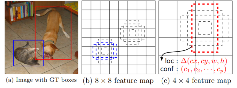The 9 anchor boxes: It have 3 aspect ratios of sizes 1/2, 1 and 2. For each size, there are 3 scales. These anchors of the appropriate sizes are generated for each of 5 feature maps.

Let’s take a look at the DataEncoder class, DataEncoder.__init__:

def __init__(self, input_size):
        self.input_size = input_size
        self.anchor_areas = [8 * 8, 16 * 16., 32 * 32., 64 * 64., 128 * 128]  # p3 -> p7
        self.aspect_ratios = [0.5, 1, 2]
        self.scales = [1, pow(2, 1 / 3.), pow(2, 2 / 3.)]
        num_fms = len(self.anchor_areas)
        fm_sizes = [math.ceil(self.input_size[0] / pow(2., i + 3)) for i in range(num_fms)]
        self.anchor_boxes = []
        for i, fm_size in enumerate(fm_sizes):
            anchors = generate_anchors(self.anchor_areas[i], self.aspect_ratios, self.scales)
            anchor_grid = generate_anchor_grid(input_size, fm_size, anchors)
            self.anchor_boxes.append(anchor_grid)
        self.anchor_boxes = torch.cat(self.anchor_boxes, 0)
        self.classes = ["__background__", "person"]

As seen, it chose the anchor area which is responsible for generating anchors for the output layer of FPN.
256/8 = 32 # first is for generating achchors for 1st FPN output layer
256/16 = 16
.
.
256/128 = 2
To generate 9 anchors, using predefined ratios and scales.

def generate_anchors(anchor_area, aspect_ratios, scales):
    anchors = []
    for scale in scales:
        for ratio in aspect_ratios:
            h = math.sqrt(anchor_area/ratio)
            w = math.sqrt(anchor_area*ratio)
            x1 = (math.sqrt(anchor_area) - scale * w) * 0.5
            y1 = (math.sqrt(anchor_area) - scale * h) * 0.5
            x2 = (math.sqrt(anchor_area) + scale * w) * 0.5
            y2 = (math.sqrt(anchor_area) + scale * h) * 0.5
            anchors.append([x1, y1, x2, y2])
    return torch.Tensor(anchors)

for each feature map, a grid will be created, which will allow all the possible box.

def generate_anchor_grid(input_size, fm_size, anchors):
    grid_size = input_size[0] / fm_size
    x, y = torch.meshgrid(torch.arange(0, fm_size) * grid_size, torch.arange(0, fm_size) * grid_size)
    anchors = anchors.view(-1, 1, 1, 4)
    xyxy = torch.stack([x, y, x, y], 2).float()
    boxes = (xyxy + anchors).permute(2, 1, 0, 3).contiguous().view(-1, 4)
    boxes[:, 0::2] = boxes[:, 0::2].clamp(0, input_size[0])
    boxes[:, 1::2] = boxes[:, 1::2].clamp(0, input_size[1])
    return boxes

Next check the size of anchor boxes by input different image size:

height_width = (256, 256)
data_encoder = DataEncoder(height_width)
print('anchor_boxes size: {}'.format(data_encoder.anchor_boxes.size()))

anchor_boxes size: torch.Size([12276, 4])

height_width = (300, 300)
data_encoder = DataEncoder(height_width)
print('anchor_boxes size: {}'.format(data_encoder.anchor_boxes.size()))

anchor_boxes size: torch.Size([17451, 4])

So to compare the anchor boxes size with network output size:

Image input size	Anchor boxes size	Detector Network output size
(256, 256)	[12276, 4]	[batch_size, 12276, 4]
(300, 300)	[17451, 4]	[batch_size, 17451, 4]

Basically, we want to encode the location target so that the size of location target becomes equal to the size of anchor boxes.

Matching Predictions with Ground Truth

After having a wide range of anchors, we want to know which of them are the most suitable for training. By computing the intersection over union (IoU) between anchors and target boxes, those boxes that will have the maximum metric will be used further in training.
If anchor box’s IoU is in between 0.4 and 0.5, it can be considered as a bad match with the target and ignore it in the training process;
If anchor box’s IoU is below 0.4, it can be considered as background;
After that, all of the matched boxes should be encoded.

def encode(self, boxes, classes):
        iou = compute_iou(boxes, self.anchor_boxes)
        iou, ids = iou.max(1)
        loc_targets = encode_boxes(boxes[ids], self.anchor_boxes)
        cls_targets = classes[ids]
        cls_targets[iou < 0.5] = -1
        cls_targets[iou < 0.4] = 0

        return loc_targets, cls_targets

Encoding Boxes Instead of predicting the bounding box location on the image directly, the bounding box regressor predicts the offset of the bounding box to anchor boxes. Representing the bounding box with respect to anchor boxes requires encoding.
Generally a bounding box is presented in [𝑥𝑚𝑖𝑛,𝑦𝑚𝑖𝑛,𝑥𝑚𝑎𝑥,𝑦𝑚𝑎𝑥] format. However, at the time of learning these boxes, it learns the bounding boxes with respect to nearby anchors.

def encode_boxes(boxes, anchors):
    anchors_wh = anchors[:, 2:] - anchors[:, :2] + 1  # width and height
    anchors_ctr = anchors[:, :2] + 0.5 * anchors_wh   # center of the bounding box
    boxes_wh = boxes[:, 2:] - boxes[:, :2] + 1
    boxes_ctr = boxes[:, :2] + 0.5 * boxes_wh
    return torch.cat([(boxes_ctr - anchors_ctr) / anchors_wh, torch.log(boxes_wh / anchors_wh)], 1)

Precisely, it is encoded as follows:

Difference between center co-ordinates of the nearby anchors and the ground truth bounding box, divided by the anchor width-height. (boxes_ctr - anchors_ctr) / anchors_wh
Logs of width and height ratio. torch.log(boxes_wh / anchors_wh)

Training is trying to learn how to move the predicted box to look the same as the target. For that purpose, we should encode anchors as the offsets to the target bounding boxes which need to learn.

The offset is calculated with respect to the center of the box and includes how the width and the height should be regressed. Concatenate along axis-1 by using torch.cat([(boxes_ctr - anchors_ctr) / anchors_wh, torch.log(boxes_wh / anchors_wh)], 1). This is the encoded format of bounding boxes.

Decoding Boxes In order to obtain the boxes as standard format:

def decode_boxes(deltas, anchors):
 if torch.cuda.is_available():
     anchors = anchors.cuda()
 anchors_wh = anchors[:, 2:] - anchors[:, :2] + 1
 anchors_ctr = anchors[:, :2] + 0.5 * anchors_wh
 pred_ctr = deltas[:, :2] * anchors_wh + anchors_ctr
 pred_wh = torch.exp(deltas[:, 2:]) * anchors_wh
 return torch.cat([pred_ctr - 0.5 * pred_wh, pred_ctr + 0.5 * pred_wh - 1], 1)

Note that the classification choose threshold 0.5 to not consider all of the predictions with lower probabilities. Even after thresholding, some bounding boxes with similar box coordinates need to be suppressed. To remove this redundancy, vanilla non-maximum-suppression (NMS) should be applied.

 def decode(self, loc_pred, cls_pred, cls_threshold=0.7, nms_threshold=0.3):
        all_boxes = [[] for _ in range(len(loc_pred))]  # batch_size

        for sample_id, (boxes, scores) in enumerate(zip(loc_pred, cls_pred)):
            boxes = decode_boxes(boxes, self.anchor_boxes)

            conf = scores.softmax(dim=1)
            sample_boxes = [[] for _ in range(len(self.classes))]
            for class_idx, class_name in enumerate(self.classes):
                if class_name == '__background__':
                    continue
                class_conf = conf[:, class_idx]
                ids = (class_conf > cls_threshold).nonzero().squeeze()
                ids = [ids.tolist()]
                keep = compute_nms(boxes[ids], class_conf[ids], threshold=nms_threshold)

                conf_out, top_ids = torch.sort(class_conf[ids][keep], dim=0, descending=True)
                boxes_out = boxes[ids][keep][top_ids]

                boxes_out = boxes_out.cpu().numpy()
                conf_out = conf_out.cpu().numpy()

                c_dets = np.hstack((boxes_out, conf_out[:, np.newaxis])).astype(np.float32, copy=False)
                c_dets = c_dets[c_dets[:, 4].argsort()]
                sample_boxes[class_idx] = c_dets

            all_boxes[sample_id] = sample_boxes

        return all_boxes

Loss Function

Object detector has 2 branches with 2 independent outputs. At each iterations, need to address: 1. how close are the predicted bounding boxes to the target bounding boxes, and 2. whether their labels are predicted correctly.

Hence, Loss function is represented as a sum of two losses: localization and classification loss.

class DetectionLoss(nn.Module):
    def __init__(self, num_classes=2):
        super().__init__()
        self.num_classes = num_classes

    def forward(self, loc_preds, loc_targets, cls_preds, cls_targets):
        '''Compute loss between (loc_preds, loc_targets) and (cls_preds, cls_targets).

        Args:
          loc_preds: (tensor) predicted locations, sized [batch_size, #anchors, 4].
          loc_targets: (tensor) encoded target locations, sized [batch_size, #anchors, 4].
          cls_preds: (tensor) predicted class confidences, sized [batch_size, #anchors, #classes].
          cls_targets: (tensor) encoded target labels, sized [batch_size, #anchors].

        loss:
          (tensor) loss = SmoothL1Loss(loc_preds, loc_targets) + OHEMLoss(cls_preds, cls_targets).
        '''

Localization loss

As Faster R-CNN, Smooth L1-loss is a leveraged because it solved for bounding box regression problems of L2 loss, as sensitive to outliers.

Smooth L1-loss can be interpreted as a combination of L1-Loss (when the absolute value of the argument is high) and L2-Loss (when the absolute value of the argument is close to zer).

    pos = cls_targets > 0  # [N,#anchors]
    num_pos = pos.long().sum(1, keepdim=True)

    mask = pos.unsqueeze(2).expand_as(loc_preds)  # [N,#anchors,4]
    masked_loc_preds = loc_preds[mask].view(-1, 4)  # [#pos,4]
    masked_loc_targets = loc_targets[mask].view(-1, 4)  # [#pos,4]
    loc_loss = F.smooth_l1_loss(masked_loc_preds, masked_loc_targets, reduction='none')
    loc_loss = loc_loss.sum() / num_pos.sum().float()

Classification loss

As the most popular loss for classification task, Cross Entropy is leveraged. Note that class imbalance is a very problematic issue for single-stage detectors. This is because most locations in an image are negatives, that can be easily classified by the detector as background.

So I really want the network to train on hard examples with positives, which constitute only a small part of all of the locations. To address this problem, Online Hard Example Mining (OHEM) strategy appiled. It finds hard examples in the batch with the greatest loss values and back-propagates the loss computed over the selected instances. The amount of hard examples correlates with the number of positive examples and is often chosen as 3:1.

# Compute max conf across batch for hard negative mining
batch_size, _ = cls_targets.size()
batch_conf = cls_preds.view(-1, self.num_classes)
cls_loss = F.cross_entropy(batch_conf, cls_targets.view(-1), ignore_index=-1, reduction='none')
cls_loss = cls_loss.view(batch_size, -1)

# Hard Negative Mining
# filter out pos boxes (pos = cls_targets > 0) for now.
pos_cls_loss = cls_loss[pos]
        
# In OHEM, we have to select only those background labels (0) that have been failed with 
# a very high margin (lets we will choose three times (negpos_ratio = 3) of the object labels (>=1)). 
        
# To paly around background labels, let's make zero loss to object labels.
cls_loss[pos] = 0 
        
# Let's find indices of decreasing order of loss (which ground truth is background). 
_, loss_idx = cls_loss.sort(1, descending=True)
        
# If we sort (in increasing order) the above indices, indices correspond to the sorting will 
# give a ranking (along dimension 1) of the original loss matrix. 
_, idx_rank = loss_idx.sort(1)
        
# Let's understand by example. As all operations are along axis 1, taking 1-d example will be sufficient.
# cls_loss = [5, 2, 9, 6,  8]
# _, loss_idx = cls_loss.sort(descending=True)
# loss_idx = [2, 4, 3, 0, 1]

# _, idx_rank = loss_idx.sort()
# idx_rank = [3, 4, 0, 2, 1]
        
# Have a look, idx_rank has the ranking of cls_loss.
negpos_ratio = 3
        
# We have decided we will take the negative class count three times of the positive class. 

# If we do it blindly, in the case of not a positive class in the image, we will end up missing 
# all the negative class also. So let's clamp minimum to 1. 
# Although maximum clamping is not required here,  let fix to maximum index. 

num_neg = torch.clamp(negpos_ratio * num_pos, min=1, max=pos.size(1) - 1)

neg = idx_rank < num_neg.expand_as(idx_rank)
neg_cls_loss = cls_loss[neg]

cls_loss = (pos_cls_loss.sum() + neg_cls_loss.sum()) / num_pos.sum().float()
       

Training

%matplotlib notebook
%load_ext autoreload
%autoreload 2

import os
import random

from operator import itemgetter

import cv2
import numpy as np
import torch
import torch.optim as optim
import matplotlib.pyplot as plt

from albumentations import (
    CLAHE,
    Blur,
    OneOf,
    Compose,
    RGBShift,
    GaussNoise,
    RandomGamma,
    RandomContrast,
    RandomBrightness,
)

from torch.utils.data import DataLoader
from torch.optim.lr_scheduler import MultiStepLR
from albumentations.pytorch.transforms import ToTensorV2
from albumentations.augmentations.transforms import HueSaturationValue
from albumentations.augmentations.transforms import Normalize

from trainer import Trainer, hooks, configuration
from detector import Detector
from trainer.utils import patch_configs
from trainer.utils import setup_system
from detection_loss import DetectionLoss
from trainer.encoder import (
    DataEncoder,
    decode_boxes,
    encode_boxes,
    generate_anchors,
    generate_anchor_grid,
)
from trainer.metrics import APEstimator
from trainer.datasets import ListDataset
from trainer.data_set_downloader import DataSetDownloader 
from trainer.matplotlib_visualizer import MatplotlibVisualizer

class Experiment:
    def __init__(
        self,
        system_config: configuration.SystemConfig = configuration.SystemConfig(),
        dataset_config: configuration.DatasetConfig = configuration.DatasetConfig(),  # pylint: disable=redefined-outer-name
        dataloader_config: configuration.DataloaderConfig = configuration.DataloaderConfig(),  # pylint: disable=redefined-outer-name
        optimizer_config: configuration.OptimizerConfig = configuration.OptimizerConfig(),  # pylint: disable=redefined-outer-name
    ):
        self.system_config = system_config
        setup_system(system_config)
        self.dataset_train = ListDataset(
            root_dir=dataset_config.root_dir,
            list_file='../train_anno.txt',
            classes=["__background__", "person"],
            mode='train',
            transform=Compose(dataset_config.train_transforms),
            input_size=300
        )

        self.loader_train = DataLoader(
            dataset=self.dataset_train,
            batch_size=dataloader_config.batch_size,
            shuffle=True,
            collate_fn=self.dataset_train.collate_fn,
            num_workers=dataloader_config.num_workers,
            pin_memory=True
        )

        self.dataset_test = ListDataset(
            root_dir=dataset_config.root_dir,
            list_file='../test_anno.txt',
            classes=["__background__", "person"],
            mode='val',
            transform=Compose([Normalize(), ToTensorV2()]),
            input_size=300
        )
        self.loader_test = DataLoader(
            dataset=self.dataset_test,
            batch_size=dataloader_config.batch_size,
            shuffle=False,
            collate_fn=self.dataset_test.collate_fn,
            num_workers=dataloader_config.num_workers,
            pin_memory=True
        )
        self.model = Detector(len(self.dataset_train.classes))
        self.loss_fn = DetectionLoss(len(self.dataset_train.classes))
        self.metric_fn = APEstimator(classes=self.dataset_test.classes)
        self.optimizer = optim.SGD(
            self.model.parameters(),
            lr=optimizer_config.learning_rate,
            weight_decay=optimizer_config.weight_decay,
            momentum=optimizer_config.momentum
        )
        self.lr_scheduler = MultiStepLR(
            self.optimizer, milestones=optimizer_config.lr_step_milestones, gamma=optimizer_config.lr_gamma
        )
        self.visualizer = MatplotlibVisualizer()

    def run(self, trainer_config: configuration.TrainerConfig):
        setup_system(self.system_config)
        device = torch.device(trainer_config.device)
        self.model = self.model.to(device)
        self.loss_fn = self.loss_fn.to(device)

        model_trainer = Trainer(
            model=self.model,
            loader_train=self.loader_train,
            loader_test=self.loader_test,
            loss_fn=self.loss_fn,
            metric_fn=self.metric_fn,
            optimizer=self.optimizer,
            lr_scheduler=self.lr_scheduler,
            device=device,
            data_getter=itemgetter("image"),
            target_getter=itemgetter("target"),
            stage_progress=trainer_config.progress_bar,
            get_key_metric=itemgetter("mAP"),
            visualizer=self.visualizer,
            model_save_best=trainer_config.model_save_best,
            model_saving_frequency=trainer_config.model_saving_frequency,
            save_dir=trainer_config.model_dir
        )

        model_trainer.register_hook("train", hooks.train_hook_detection)
        model_trainer.register_hook("test", hooks.test_hook_detection)
        model_trainer.register_hook("end_epoch", hooks.end_epoch_hook_detection)
        self.metrics = model_trainer.fit(trainer_config.epoch_num)
        return self.metrics

    def draw_bboxes(self, rows, columns, trainer_config: configuration.TrainerConfig):
        # load the best model
        if trainer_config.model_save_best:
            self.model.load_state_dict(
                torch.
                load(os.path.join(trainer_config.model_dir, self.model.__class__.__name__) + '_best.pth')
            )
        # or use the last saved
        self.model = self.model.eval()

        std = (0.229, 0.224, 0.225)
        mean = (0.485, 0.456, 0.406)

        std = torch.Tensor(std)
        mean = torch.Tensor(mean)

        fig, ax = plt.subplots(
            nrows=rows, ncols=columns, figsize=(10, 10), gridspec_kw={
                'wspace': 0,
                'hspace': 0.05
            }
        )

        for axi in ax.flat:
            index = random.randrange(len(self.loader_test.dataset))

            image, gt_boxes, _ = self.loader_test.dataset[index]

            device = torch.device(trainer_config.device)
            image = image.to(device).clone()

            loc_preds, cls_preds = self.model(image.unsqueeze(0))

            with torch.no_grad():
                img = image.cpu()
                img.mul_(std[:, None, None]).add_(mean[:, None, None])
                img = torch.clamp(img, min=0.0, max=1.0)
                img = img.numpy().transpose(1, 2, 0)

                img = (img * 255.).astype(np.uint8)
                gt_img = img.copy()
                pred_img = img.copy()

                for box in gt_boxes:
                    gt_img = cv2.rectangle(
                        gt_img, (int(box[0]), int(box[1])), (int(box[2]), int(box[3])), (255, 0, 0),
                        thickness=2
                    )

                encoder = DataEncoder((img.shape[1], img.shape[0]))
                samples = encoder.decode(loc_preds, cls_preds)
                c_dets = samples[0][1]  # detections for class == 1

                if c_dets.size > 0:
                    boxes = c_dets[:, :4]
                    for box in boxes:
                        pred_img = cv2.rectangle(
                            pred_img, (int(box[0]), int(box[1])), (int(box[2]), int(box[3])), (0, 0, 255),
                            thickness=2
                        )

                merged_img = np.concatenate((gt_img, pred_img), axis=1)
                axi.imshow(merged_img)
                axi.axis('off')
        fig.show()


if __name__ == '__main__':
    dataloader_config, trainer_config = patch_configs(epoch_num_to_set=100, batch_size_to_set=30)
    # Downloading dataset
    DataSetDownloader(root_dir='data', dataset_title='PennFudanPed', download=True)
    dataset_config = configuration.DatasetConfig(
        root_dir="data/PennFudanPed/",
        train_transforms=[
            RandomBrightness(p=0.5),
            RandomContrast(p=0.5),
            OneOf([
                RandomGamma(),
                HueSaturationValue(hue_shift_limit=20, sat_shift_limit=50, val_shift_limit=50),
                RGBShift()
            ],
                p=1),
            OneOf([Blur(always_apply=True), GaussNoise(always_apply=True)], p=1),
            CLAHE(),
            Normalize(),
            ToTensorV2()
        ]
    )
    
    optimizer_config = configuration.OptimizerConfig(
        learning_rate=5e-3, 
        lr_step_milestones=[50], 
        lr_gamma=0.1, 
        momentum=0.9, 
        weight_decay=1e-5
    )
    
    experiment = Experiment(
        dataset_config=dataset_config, 
        dataloader_config=dataloader_config, 
        optimizer_config=optimizer_config
    )
    
    # Run the experiment / start training
    experiment.run(trainer_config)
    
    # how good our detector works by visualizing the results on the randomly chosen test images:
    experiment.draw_bboxes(4, 1, trainer_config)

"Create a custom single-stage detector"